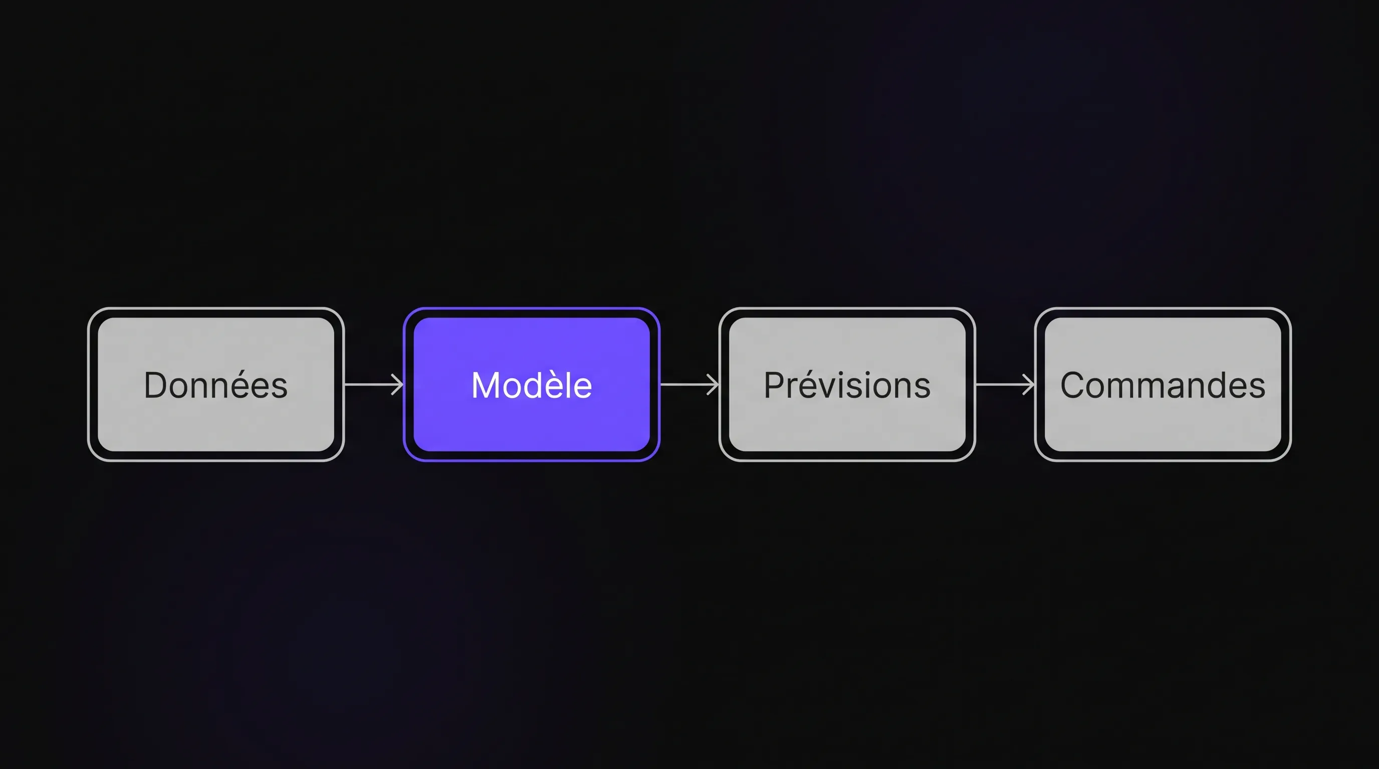
Artificial Intelligence and Machine Learning for Demand Forecasting
Intelligence artificielle
Stratégie d'entreprise
Optimisation
Sales
Discover how SMEs can leverage AI and machine learning for demand forecasting to balance inventory, reduce stockouts, and turn data into smart purchasing decisions.
October 28, 2026·14 min read
Behind the search for "artificial intelligence machine learning," an operational question arises for SMEs: how can you anticipate orders without tying up too much cash or multiplying stockouts? Forecasting demand means estimating what customers will want to buy over an actionable time horizon.
AI can help uncover patterns and leverage multiple signals, but it replaces neither reliable data nor a well-defined procurement decision. The goal is not to produce an impressive curve. It is to make better decisions on what to order, when, and in what quantities, while accounting for explicit uncertainty. This also applies to forecasting service workloads or the hiring needs of a growing team.
"Artificial Intelligence Machine Learning": Understanding What Is Being Forecast
Artificial intelligence refers to a set of methods that enable a system to accomplish tasks such as recognizing patterns, classifying, or forecasting. Machine learning is a branch of AI: models learn relationships from examples rather than relying exclusively on hand-crafted rules.
To forecast sales, supervised learning is generally used. The model connects information available at a given date to a quantity observed later. Unsupervised learning can cluster products with similar behaviors. Reinforcement learning focuses on sequential decision-making and is usually not the starting point for a forecasting project.
Deep learning relies on neural networks and is also part of machine learning. It is not strictly necessary for an SME. A statistical model or a simpler algorithm may be better suited to its historical data.
Demand does not always equal recorded sales. An out-of-stock item may show zero sales even if customers wanted to buy it. Confusing the two leads to repeating stockouts.
Start from the Decision, Not the Algorithm
Before combining artificial intelligence and machine learning, specify the decision you want to improve. A distributor waiting three weeks for a delivery should not just forecast the next day's sales. Its horizon must cover the time required to react.
Define the expected quantity, the level of granularity, and the update frequency. A weekly forecast by category helps prepare a budget. A forecast by SKU and warehouse is more useful for replenishment. For team scheduling, the relevant variable might instead be a volume of tickets or service interventions.
The right level of precision also depends on available volume. Breaking down a few monthly orders by product, channel, and region can create series that are too sparse to be useful. It is sometimes better to forecast at an aggregate level, then allocate using a transparent rule.
Finally, establish the economic trade-offs: lost margin during stockouts, holding costs, obsolescence risk, and operational capacity. A company selling perishable goods penalizes an overestimation differently than a critical spare parts supplier penalizes an underestimation. These choices determine what a "good" forecast actually means.
Actionable Data, Not Just Sales History
A project combining artificial intelligence and machine learning starts with reliable data. Priority data includes dated orders or sales, quantities, SKUs, and sales locations. Add available inventory, returns, prices, and promotions when this information is dependable. Supplier lead times are necessary to turn forecasts into orders.
Keep track of stockout periods. A lack of sales due to unavailability must not be interpreted as a drop in customer interest. Any correction for unobserved demand should be documented: lost sales remain an estimate, not a reconstructed ground truth.
Calendars often provide useful variables: business days, holidays, school breaks, and known events. Weather may matter in certain industries, but only weather forecasts actually available at decision time should enter a realistic historical simulation.
No universal number of months of history guarantees success. Several cycles make it easier to analyze annual seasonality; a few months do not allow for solid measurement. Historical data may also become unrepresentative following a major business shift.
Finally, check for duplicates, units of measurement, SKU changes, and the distinction between missing values and zeros. A canceled order or a misinterpreted ERP migration can degrade a forecast more than a poor choice of algorithm.
Running Example: An SME and 300 SKUs
Let us take a fictional example: an e-commerce SME sells 300 home accessory SKUs. It has 30 months of daily sales data, with shorter histories for certain products. Supplier orders are reviewed weekly, and the standard lead time is two weeks.
The project does not start across the entire catalog. The team selects a product family with usable history and an identified inventory challenge. They aggregate sales by week, reconcile stock availability, and record scheduled promotions.
In this case, artificial intelligence and machine learning serve to estimate volumes for the next three weeks: two weeks of lead time plus one week until the next review cycle. The forecast will be compared against the current baseline method, not just human intuition.
The dataset contains one row per SKU and week, with a target quantity. Variables might include sales from previous weeks, a recent rolling average, price, and the known promotional calendar. New SKUs remain handled separately as long as their history is too short.
Choose the Simplest Model That Beats the Baseline
Start with a simple baseline: repeat the previous week, use a moving average, or reproduce a comparable week from the previous year when relevant. These approaches are mandatory benchmarks, not embarrassments to hide.
Statistical time series models, such as exponential smoothing, suit certain trend and seasonality profiles. Regression and tree-based ensembles, particularly gradient boosting, make it possible to factor in multiple drivers. Their added value must be demonstrated on your data.
A model shared across multiple SKUs can learn common patterns. Conversely, intermittent demand, characterized by long periods without sales, requires specific evaluation and sometimes dedicated methods. No single algorithm wins in every situation.
Combining artificial intelligence and machine learning does not mandate a neural network. If a moving average yields equally sound decisions with lower maintenance, keep it. Our guide on the differences between deterministic rules and AI helps clarify this boundary.
A generative model can explain a result or structure commercial information. It does not replace an evaluated numerical forecasting system on its own.
Test Without Letting the Future Leak into the Past
Randomly splitting rows is generally unsuitable for time series. It can allow future information to contaminate model training. Validation must reproduce operational reality: at each decision date, the model only knows what was available at that point in time.
For our fictional SME, parameters are tuned on earlier windows. The final twelve weeks are kept aside as a test set. Evaluation covers one-, two-, and three-week horizons, because a good short-term forecast does not guarantee good replenishment planning.
This short test window does not necessarily cover all seasons. If holiday sales drive most of your business, evaluate comparable windows from prior years and flag periods where you lack sufficient historical depth.
In an artificial intelligence and machine learning setup, data leakage is often subtle. A promotion decided after the simulated date, stock adjusted retroactively, or an average calculated using future sales can artificially inflate performance.
Apply data preprocessing steps exclusively to the training sets. Document information that was unavailable at the time rather than creating an artificially sanitized past.
Measure Error, Bias, and Business Outcomes
A single average error metric is not enough. Examine its magnitude, direction, and distribution across products. Bias reveals a tendency to systematically over- or under-forecast; offsetting errors can cancel each other out without yielding satisfactory decisions.
Here are three fictional weeks for a single SKU:
Week
Actual Sales
Forecast
Absolute Error
1
100
100
0
2
120
110
10
3
80
90
10
The total actual volume is 300 units, and the cumulative absolute error is 20. WAPE, calculated here as the sum of absolute errors divided by the sum of actual quantities, is approximately 6.7%. Overall bias is zero: total forecasted and actual volumes match, despite two individual errors.
WAPE cannot be calculated when total demand is zero and favors high-volume SKUs in an aggregated evaluation. MAPE also breaks down with zero sales. Supplement these metrics with unit-level absolute error and segmented analysis.
Also check consistency across hierarchy levels: SKU-level forecasts should align with category and catalog totals. An overall improvement can hide performance drops on a strategic SKU, even if its sales volume is low.
To judge artificial intelligence and machine learning, monitor stockouts, average inventory, and an explicitly defined service level. These outcomes also depend on suppliers and reordering policies: improved accuracy alone does not prove an operational gain.
Turn a Forecast into an Order Quantity
A forecast estimates demand. An inventory policy turns that estimate into action, factoring in on-hand inventory, open orders, lead times, and purchasing constraints. This connection is what makes artificial intelligence and machine learning valuable day to day.
Let us return to our SME with a weekly review and a fixed two-week lead time. For one SKU, the forecasts for the next three weeks are 100, 110, and 90 units. Total expected demand across the protection period is 300 units.
Assume, strictly for illustrative purposes, a safety stock of 60 units. The target inventory position is 360 units. The company has 180 units in stock, expects 80 units already ordered, and has 20 backordered units still to fulfill.
Its net stock position is 180 + 80 - 20 = 240 units. The proposed order quantity is therefore 360 - 240 = 120 units, before applying minimum order quantities, packaging multiples, and budget constraints.
Safety stock should not be picked arbitrarily in production. It depends on the target service level, forecast error over the relevant horizon, and lead time variability. Arrival schedules must also be verified: a late delivery will not cover an immediate stockout.
Handle Demand Spikes, New Launches, and Uncertainty
A single-point value hides uncertainty. When the tool supports it, pair a central forecast with prediction intervals or quantiles, and validate their calibration on out-of-sample data. An 80% interval should contain approximately 80% of actual outcomes in comparable situations.
Exceptional promotions, price changes, or product launches require explicit handling. If historical data contains no comparable events, the model cannot infer a reliable effect. Prepare multiple scenarios and document commercial assumptions.
For new products, consider using reference analogues or shared attributes, while acknowledging higher uncertainty. Rapid business growth also requires distinguishing sustained trends from temporary spikes.
In these scenarios, artificial intelligence and machine learning inform decisions without replacing business judgment. Manual overrides should be documented, dated, and later compared against actual results to verify whether they genuinely improve decisions.
Embed Forecasts into Daily Workflows
A forecast delivered in an overlooked spreadsheet changes nothing in how a business operates. Define where it surfaces: an ERP, an internal business tool, or a replenishment interface. The end user needs to see the relevant period, key assumptions, and the last update date.
The process can follow a weekly cadence: ingest new data, validate consistency, generate forecasts, and compute purchase recommendations. Missing data or anomalous volumes should trigger an alert rather than a silent failure.
Initially, keep human validation in the loop for purchase orders. Broader automation can be phased in over a controlled scope, bounded by quantity or budget caps. Maintain a fallback rule if the model or data pipeline fails.
Integrating artificial intelligence and machine learning requires as much clarity around roles as around code. Designate who inspects anomalies and who approves overrides. Our guide on choosing, integrating, and measuring an AI solution breaks down this transition from requirement to adoption.
Run a Pilot on a Limited Scope
A pilot must test an end-to-end decision, not just train an algorithm. Select a scope where data is accessible, users are available, and business stakes are measurable. A single product family is sufficient if it reflects real operational dynamics without bundling every edge case.
Define clear go/no-go criteria upfront: improvement over the baseline, no performance degradation on sensitive segments, and manageable maintenance overhead. Thresholds depend on your costs and risk tolerance; they are not universal.
Run recommendations in parallel with the current process before changing actual purchase orders. This phase highlights missing data, overlooked supplier constraints, and interpretation issues.
However, shadow testing alone does not measure stockout reductions: as long as decisions remain unchanged, that benefit is simulated. A phased rollout, using a control group where possible, provides a more reliable operational evaluation.
To compare two methods fairly, maintain identical lead times, purchasing constraints, and inventory policies in the simulation. Otherwise, you risk attributing the impact of a logistical or pricing policy change to the forecasting model. Document forecast adjustments and order adjustments separately.
Calculate ROI Using Total Cost of Ownership
The return on investment of an artificial intelligence and machine learning initiative is not measured simply in percentage points of error reduction. It depends on the decisions actually changed and the total cost of ownership.
Estimate preserved margin from prevented lost sales, reduced holding costs, fewer markdowns, and saved planning time. Avoid double counting: lower inventory frees up cash, but that one-off cash release is not recurring annual profit.
Conversely, factor in data preparation, connectors, custom development or licenses, hosting, monitoring, and team time. A slightly less accurate model can deliver a better bottom line if it is simpler to operate.
Finally, compare multiple economic scenarios rather than assuming a single projected gain. If expected benefits remain below ongoing maintenance costs, a well-tuned replenishment rule is already a worthwhile improvement.
Protect Data and Maintain Long-Term Reliability
Forecasting by product or store rarely requires customer identities. Work with aggregated data whenever possible and limit the information shared with external vendors. If personal data is involved, specify the purpose, legal basis, access rights, and retention periods in accordance with GDPR.
The CNIL provides guidance on artificial intelligence to help navigate these requirements. Aggregation does not automatically guarantee anonymity: small group sizes or cross-referencing can still allow re-identification.
Also review hosting contract terms, commercial data confidentiality, and provisions for data deletion or return at the end of the engagement.
Reliability also demands post-deployment monitoring. Changes in product catalogs, sales channels, or customer buying behavior can degrade learned patterns. Track error, bias, missing inputs, and manual overrides, and retrain the model when warranted.
Finally, prevent the system from amplifying its own errors: under-forecasting an item reduces reorders, lowering observed sales. Without tracking stockouts, the model may misinterpret that decline as falling demand.
Frequently Asked Questions
Do you need massive amounts of data to start? You primarily need data consistent with your decision cadence. The required history depends on seasonality, sales frequency, and business changes. Start by measuring what a simple baseline method can already achieve.
Can you forecast demand with ChatGPT? A generative assistant can help explore a file or structure an analysis. Its raw answers alone do not constitute a validated forecasting system. Calculations must rely on controlled data pipelines and chronological testing.
When does machine learning become worthwhile? When it beats a simple baseline on simulated future data, providing a tangible decision-making benefit. Having multiple demand drivers, such as pricing and promotions, can justify testing ML without guaranteeing success.
Can purchasing be automated from day one? It is better to start with human approval, explicit thresholds, and a fallback procedure. Automation should scale with proven reliability and the cost of errors.
Scope Your First Forecasting Use Case
Before picking a technology, gather a representative historical sample, define the decision to improve, and benchmark your current baseline method. This foundation lets you evaluate whether artificial intelligence and machine learning deliver a measurable advantage.
Impulse Lab helps companies with AI opportunity audits, custom web and AI development, system integrations, and team training. For your forecasting project, start by scoping the operational need and data quality before deciding what to build.